Linear regression from scratch with tf.GradientTape
TensorFlow’s GradientTape is a context manager for automatic differentiation. To understand how it works a bit better, here I have implemented a linear regression from scratch using it.
Before we get to that though, let’s quickly look at the syntax for computing gradients:
import tensorflow as tf

x = tf.Variable(3.0)

with tf.GradientTape() as tape:
    y = x**2

tape.gradient(y, x)
<tf.Tensor: id=552560, shape=(), dtype=float32, numpy=6.0>
As you can see, this is fairly straghtforward, the gradient method is invoked to compute the gradient of the target (in our case y) with respect to the sources (x).
So now let’s implement a simple linear regression from scratch using GradientTape for our gradient descent. First we can define some simple helper functions to compute the loss, compute the gradients and update the weights.
def loss_mse(X, Y, w0, w1):
    """Compute mean squared error"""
    Y_hat = w0 * X + w1
    errors = (Y_hat - Y)**2
    return tf.reduce_mean(errors)

def compute_gradients(X, Y, w0, w1):
    """Compute gradient of loss function w.r.t weights"""
    with tf.GradientTape() as tape:
        loss = loss_mse(X, Y, w0, w1)
    return tape.gradient(loss, [w0, w1])

def update_weights(w0, w1, dw0, dw1, learning_rate):
    """Updates weights using gradient descent algorithm."""
    w0.assign_sub(dw0 * learning_rate)
    w1.assign_sub(dw1 * learning_rate)
    return w0, w1
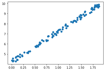
We can then create some simple linear looking data with numpy.
import numpy as np

def linear_like_data_generator(n, w0, w1):
    X = 2 * np.random.rand(n, 1)
    Y = w0 * X + w1 + 0.5 * np.random.rand(n, 1)
    return X, Y
import matplotlib.pyplot as plt

X, Y = linear_like_data_generator(100, 3, 4)

plt.scatter(X, Y)
Now we can implement gradient descent. We first set the number of steps and the learning rate we want to use. We then initialise the weights and finally we iteratively update the weights by repeating the following two steps:
- Computing the gradient of the loss function w.r.t. the weights using GradientTape.
- Updating the weights with the gradient descent algorithm
steps = 1000
learning_rate = .02

# initialise weights
w0 = tf.Variable(0.0)
w1 = tf.Variable(0.0)

# Iteratively update weights with gradient descent
for step in range(steps + 1):
    dw0, dw1 = compute_gradients(X, Y, w0, w1)
    w0, w1 = update_weights(w0, w1, dw0, dw1, learning_rate)

    # Compute loss and log stats every 100 steps
    if step % 100 == 0:
        loss = loss_mse(X, Y, w0, w1)
        print(f"STEP: {step} - loss: {loss}, w0: {w0.numpy():.4f}, w1: {w1.numpy():.4f}")
STEP: 0 - loss: 45.64582824707031, w0: 0.3233, w1: 0.2871
STEP: 100 - loss: 0.0872255340218544, w0: 3.4348, w1: 3.7167
STEP: 200 - loss: 0.03798011317849159, w0: 3.2342, w1: 3.9521
STEP: 300 - loss: 0.024118678644299507, w0: 3.1275, w1: 4.0767
STEP: 400 - loss: 0.02021694742143154, w0: 3.0709, w1: 4.1428
STEP: 500 - loss: 0.0191186610609293, w0: 3.0409, w1: 4.1779
STEP: 600 - loss: 0.01880951225757599, w0: 3.0250, w1: 4.1965
STEP: 700 - loss: 0.01872248575091362, w0: 3.0165, w1: 4.2064
STEP: 800 - loss: 0.01869799569249153, w0: 3.0120, w1: 4.2117
STEP: 900 - loss: 0.018691105768084526, w0: 3.0096, w1: 4.2144
STEP: 1000 - loss: 0.018689170479774475, w0: 3.0084, w1: 4.2159
As you can see this gets us fairly close to the “true” values of w0 and w1 of 3 and 4 respectively.